FREQUENCY Function(WS)

Description

The Microsoft Excel FREQUENCY function returns how often values occur within a set of data. It returns a vertical array of numbers.

Syntax

The syntax for the FREQUENCY function in Microsoft Excel is:

FREQUENCY( data, intervals )

Parameters or Arguments

data

An array or range of values for which to count the frequencies.

intervals

An array or range of intervals that yoiu want to group the values in data.

Applies To

• Excel 2016, Excel 2013, Excel 2011 for Mac, Excel 2010, Excel 2007, Excel 2003

Type of Function

• Worksheet function (WS)

Example (as Worksheet Function)

Let's look at some Excel FREQUENCY examples and explore how to use the FREQUENCY function as a worksheet function in Microsoft Excel.

Let's start with some easy examples.

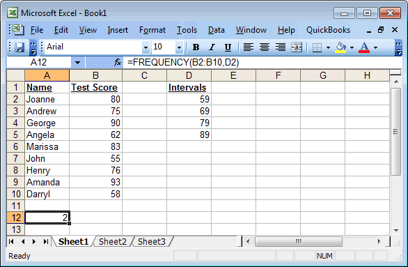
Based on the Excel spreadsheet above, the following FREQUENCY examples would return:

=FREQUENCY(B2:B10,D2)
Result: 2

=FREQUENCY(B2:B10,D3)
Result: 3

=FREQUENCY(B2:B10,D4)
Result: 5

=FREQUENCY(B2:B10,D5)
Result: 7

=FREQUENCY(B2:B10,89)
Result: 7   (same as previous)

These examples simply look at the data found in cells B2:B10 and calculate all values that are lower than the second parameter. So in the case of:

=FREQUENCY(B2:B10,D5)
Result: 7

There are 7 Test Scores in cells B2:B10 that are <= 89.

Example

Now let's take at a look at a more complex example involving array formulas.

When creating your array formula, you need to use Ctrl+Shift+Enter instead ofEnter when completing the formula. This creates {} brackets around your formula. This is very important to remember. If you do not have {} brackets around your formula, it is NOT being interpretted as an array formula by Excel.

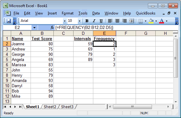
Based on the spreadsheet above, the following Excel formula{=FREQUENCY(B2:B12,D2:D5)} into cells E2:E6 using Ctrl+Shift+Enter to complete the formula. This would return a vertical array with 5 values as follows:

The first value in the array would display in cell E2. The result would be 2 (because there are 2 Test Scores <= 59).

The second value in the array would display in cell E3. The result would be 1 (because there is 1 Test Score between 60 and 69).

The third value in the array would display in cell E4. The result would be 2 (because there are 2 Test Scores between 70 and 79).

The fourth value in the array would display in cell E5. The result would be 3 (because there are 3 Test Scores between 80 and 89).

The fifth value in the array would display in cell E6. The result would be 3 (because there are 3 Test Scores > 89). This catches all values greater than the last value in the interval.

Frequently Asked Questions

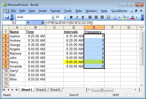
Question: In Microsoft Excel, I'm trying to use FREQUENCY to calculate the frequencies based on 5 minute intervals, but I can't seem to get the FREQUENCY function to group the values correctly. Here is a screen shot of what I have:

I'm using the formula:

{=FREQUENCY(B2:B12,D2:D9)}

As you can see, there are six "8:40:00 AM" values but they are showing up under the "8:45:00 AM" interval. Why is that?

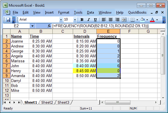
Answer: The Microsoft Excel value "8:40:00 AM" is actually stored as the numeric value 0.361111111111111 with a repeating 1. Excel must be implicity rounding the time value during its FREQUENCY calculations. To solve this problem, round the data and intervals to 13 decimal places as follows:

{=FREQUENCY(ROUND(B2:B12,13),ROUND(D2:D9,13))}

Now if we look at the results, the FREQUENCY function seems to be grouping the time intervals properly and the six "8:40:00 AM" values are showing up under the correct interval.