ISERR Function(WS)

Description

The Microsoft Excel ISERR function can be used to check for error values, except #N/A.

Syntax

The syntax for the ISERR function in Microsoft Excel is:

ISERR( value )

Parameters or Arguments

value

The value that you want to test. If value is an error value (except #N/A), this function will return TRUE. Otherwise, it will return FALSE.

Applies To

• Excel 2016, Excel 2013, Excel 2011 for Mac, Excel 2010, Excel 2007, Excel 2003, Excel XP, Excel 2000

Type of Function

• Worksheet function (WS)

Example (as Worksheet Function)

Let's look at some Excel ISERR function examples and explore how to use the ISERR function as a worksheet function in Microsoft Excel:

Based on the Excel spreadsheet above, the following ISERR examples would return:

=ISERR(A1)
Result: TRUE

=ISERR(A2)
Result: FALSE

=ISERR(A3)
Result: TRUE

=ISERR(A4)
Result: FALSE

=ISERR("www.techonthenet.com")
Result: FALSE

=ISERR(3/0)
Result: TRUE

Frequently Asked Questions

Question: Can you give me specific examples of when and how the ISERR function is used. Specifically, in a worksheet why would I use this function instead of just running down a column or across a row to look for the errors?

Answer: Often times your spreadsheet contains a large amount of formulas which will not properly calculate when an error is encountered. The ISERR function, in combination with the If function, can be used to default a cell's value when an error is occurred. This allows your formulas to evaluate properly without your intervention.

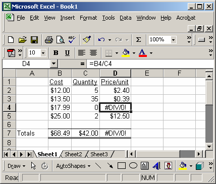
For example, you may encounter a scenario below:

Instead of using the formula:

=B4/C4

You could use the ISERR function as follows:

=IF(ISERR(B4/C4),0,B4/C4)

In this case, the ISERR function would allow you to return a 0, when an error was encounter such as a "divide by 0 error". Now all of your formulas will still work.