MS Excel 2003: Use an array formula to calculate monthly attendance

Question: In Microsoft Excel 2003/XP/2000/97, I have 2 columns. One column with "XXXXXX" which indicates a person's attendance that day and a second column indicating how many hours he was there that day. I want to compute the total hours that a person was there for a month.

How can I do this?

Answer: You can do this with an array formula.

Let's look at an example.

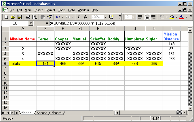
In cell E6, we want to display the total hours for Cornell. This is calculated as the sum of column L where the corresponding value in column E contains "XXXXXX". To do this, we've created the following array formula:

=SUM((E2:E5="XXXXXX")*($L$2:$L$5))

When creating your array formula, you need to use Ctrl+Shift+Enter instead of Enter. This creates {} brackets around your formula as follows:

{=SUM((E2:E5="XXXXXX")*($L$2:$L$5))}

Next, to get the total hours for Cooper, we've created the following array formula in cell F6:

{=SUM((F2:F5="XXXXXX")*($L$2:$L$5))}

And to get the total hours for Manuel, we've created the following array formula in cell G6:

{=SUM((G2:G5="XXXXXX")*($L$2:$L$5))}

And so on...