MS Excel 2010: Sort data in alphabetical order based on 2 columns

Question: In Microsoft Excel 2010, I'm trying to sort a chart that has 4 columns of data. I need to sort this data by 2 columns - first by column B (ie: Product column) in alphabetical order and then by column D (ie: Quantity) smallest to largest. How do I do this?

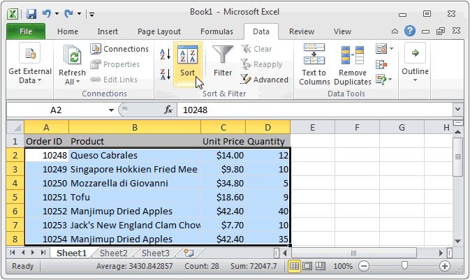
Answer: To apply this sort in Excel, highlight the data that you wish to sort. Then select theData tab from the toolbar at the top of the screen and click on the Sort button in the Sort & Filter group.

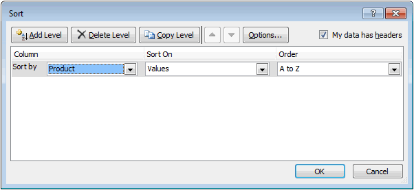
When the Sort window appears, select the first column that you wish to sort by. In this example, we want to sort by the Product column (column B) in alphabetical order (A to Z).

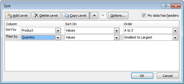
Then click on the "Add Level" button. Enter the second column that you wish to sort by. In this example, we want to sort next by the Quantity column (column D) in Smallest to Largest. Then click on the OK button.

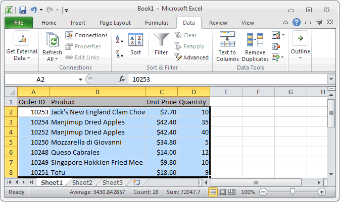
Now when you return to the spreadsheet, the data should be sorted first by Product and then by Quantity.