Add a Named Range

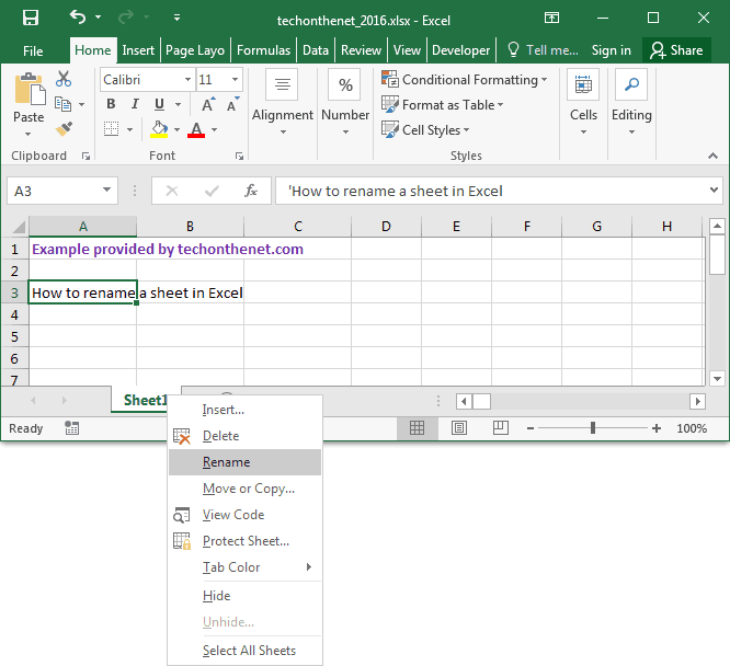
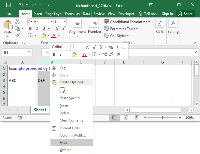
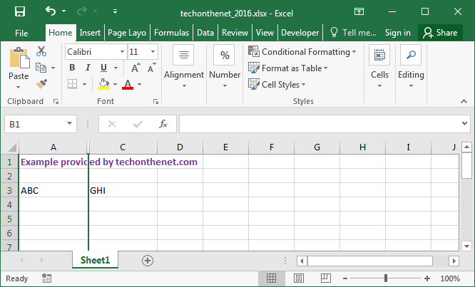
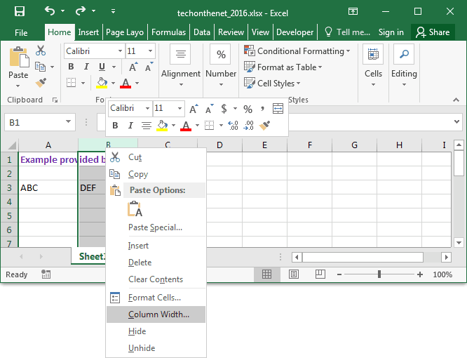
Question: In Microsoft Excel 2016, how do I set up a named range so that I can use it in a formula?

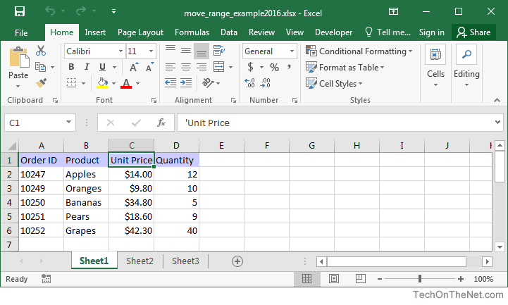
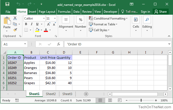
Answer: A named range is a descriptive name for a collection of cells or range in a worksheet. To add a named range, select the range of cells that you wish to name. In this example, we've selected all cells in column A.

Then select the Formulas tab in the toolbar at the top of the screen and click on the Define Name button in the Defined Names group.

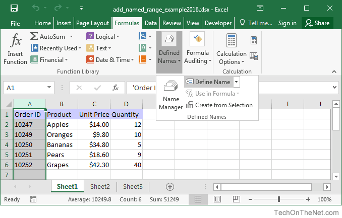
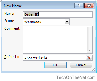
When the New Name window appears, enter a descriptive name for the range. The name can be up to 255 characters in length. In this example, we've entered Order_ID as the name for the range.

Then in the "Refers to" box, enter the range of cells that the name applies to. In this example, the range is automatically set to =Sheet1!$A:$Abecause this is the range of cells that we previously highlighted.

Then click on the OK button.

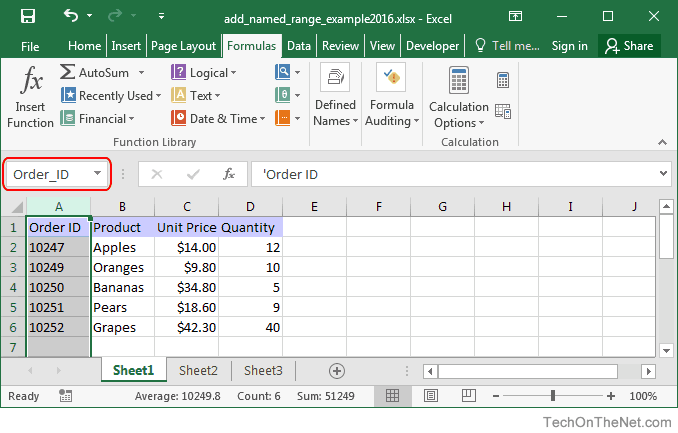
Now when you return to the spreadsheet, you will see the name Order_ID appear in the Name box (circled in red in the image below). The Name box can be found at the left end of the formula box. Now whenever you select column A, you will see this range name appear in the Name box.

Now that you have set up this named range, you can use Order_ID in formulas to refer to Column A in Sheet1.

For example:

=SUM(Order_ID)
Result: 51249

This SUM formula would add up all of the Order ID values in column A of Sheet1.

Move a Range

Question: In Microsoft Excel 2016, how do I move a range of cells along with its formatting to a different location in my spreadsheet?

Answer: By default when you move a range of cells, it will move the data as well as formatting such as font, number format, borders, background color, etc.

To move a range, select the first cell in your range. You will see the cell become active with a green box around it. In this example, we've selected cell C1.

Next, hold down the SHIFT key and click on the last cell in the range. In this example, we have clicked on cell C6. You should see the entire range of cells become highlighted.

TIP: If you want to select an entire column, click on the column letter. If you want to select an entire row, click on the row number.

Now, press CTRL + X to let Excel know that you want to move this range. You will see a dotted border appear around the range of cells indicating that the cells are ready to be moved to another location in your spreadsheet.

Next, you will need to select your destination. To do this, select the starting cell where you would like to paste the range. In this example, we have selected cell F1.

Finally, press CTRL + V to move the range (or press the ENTER key to choose Paste).

Now you should see the range move to the new location in your spreadsheet. In this example, F1:F6 now contains the original data and formatting from the range C1:C6.

Notice that your original range (C1:C6) will have all data and formatting removed.

Copy a Range

Question: In Microsoft Excel 2016, how do I copy a range of cells along with its formatting to a different location in my spreadsheet?

Answer: By default when you copy and paste and range of cells, it will copy the data as well as formatting such as font, number format, borders, background color, etc.

To copy a range, select the first cell in your range. You will see the cell become active with a black box around it. In this example, we've selected cell B1.

Next, hold down the SHIFT key and click on the last cell in the range. In this example, we have clicked on cell C6. You should see the entire range of cells become highlighted.

TIP: If you want to select an entire column, click on the column letter. If you want to select an entire row, click on the row number.

Now to copy the cells, press CTRL + C. You will see a dotted border appear around the range of cells indicating that the cells are in the clipboard and ready to be pasted to another location in your spreadsheet.

Now you will need to select your destination. To do this, select the starting cell where you would like to paste the range. In this example, we have selected cell F1.

To paste the range of cells, press CTRL + V.

Now you should see the pasted range in the new location in your spreadsheet. In this example, F1:G6 now contains a copy of the data and formatting from the range B1:C6.

Notice that your selected range (B1:C6) still has a dotted border which means that the range is still in your clipboard and you can paste it again to another location in your spreadsheet. When you are done copying and pasting the range, you can press the Escape key. This will clear the clipboard and the range will no longer be highlighted with a dotted border around it.

Delete a hyperlink from a cell

Question: How can I delete a hyperlink in Microsoft Excel 2016?

Answer:In this example, we have a hyperlink in cell A3 that we want to remove.

To remove a hyperlink from a cell, right click on the cell that has the hyperlink and select Remove Hyperlink from the popup menu.

Now when you return to the spreadsheet, you should see the hyperlink has been removed. In this example, cell A3 appears as regular text and no longer has a hyperlink.

Create a hyperlink to another cell

Question: I want to create a hyperlink in Microsoft Excel 2016. How do I specify a particular location that a hyperlink should point to?

Answer: To create a hyperlink to another cell in your spreadsheet, right click on the cell where the hyperlink should go. Select Hyperlink from the popup menu.

When the Insert Hyperlink window appears, click on the "Place In This Document" on the left. Enter the text to display. In this example, we've entered "Hyperlink to cell F4". This is the value that will be displayed in Excel.

Next enter the cell reference that the hyperlink points to. We've chosen to link to cell F4. Click the OK button.

Now when you return to the spreadsheet, you should see the hyperlink.

If you click on the hyperlink, your active cell should become cell F4.

Unhide a sheet

Question: In Microsoft Excel 2016, how do I unhide a sheet that has been hidden?

Answer: You can view all of the sheet names as tabs along the bottom of the document. In this example, Sheet2 is hidden. This is the sheet that we want to unhide.

To unhide Sheet2, right-click on the name of any sheet and select Unhide from the popup menu.

When the Unhide window appears, it will list all of the hidden sheets. Select the sheet that you wish to unhide. In this example, we've selected Sheet2. Click on the OK button.

Now when you return to your spreadsheet, Sheet2 should be visible.

Hide a sheet

Question: In Microsoft Excel 2016, how do I hide a sheet from being displayed?

Answer: You can view all of the sheet names as tabs along the bottom of the document. To hide a sheet, simply right-click on the name of the sheet that you wish to hide. In this example, we want to hide Sheet1 from being displayed.

Then select Hide from the popup menu.

Now when you return to your spreadsheet, Sheet1 should no longer be visible.

Rename a sheet

Question:In Microsoft Excel 2016, how do I rename a sheet in a spreadsheet?

Answer:You can view all of the sheet names as tabs along the bottom of the document. To rename a sheet, simply right-click on the name of the sheet that you wish to rename. In this example, we want to rename Sheet1.

Then select Rename from the popup menu.

The sheet name should now be highlighted and editable.

Enter the new name for the sheet and press the enter key on the keyboard when finished. In this example, we've renamed Sheet1 to Example.

Delete a sheet

Question:In Microsoft Excel 2016, how do I delete a sheet in a spreadsheet?

Answer:You can view all of the sheet names as tabs along the bottom of the document. To delete a sheet, simply right-click on the name of the sheet that you wish to delete. In this example, we want to delete Sheet1.

Then select Delete from the popup menu.

A message will pop up asking you to confirm the deletion of the sheet. Click on the Delete button to continue.

Now when you return to the spreadsheet, the sheet will be deleted. In this example, Sheet1 is now removed from the document.

Insert a sheet

Question: How do I insert a new sheet in Microsoft Excel 2016?

Answer: When you create a new document in Excel 2016, your spreadsheet will be created with only one worksheet called Sheet1. You can easily add more sheets as you need them.

You can view all of the sheet names as tabs along the bottom of the document. To add a new sheet, simply click on the plus button  to the right of the sheet names (we have circled this button on the image below). When you click on this plus button, it will insert a new sheet to the right of the current sheet.

Now when you return to your spreadsheet, a new sheet should be inserted and you will be positioned on cell A1 within this new sheet. In this example, Sheet2 has been inserted into the spreadsheet. Excel will always name its sheets as Sheet1, Sheet2, Sheet3, and so on.

Unhide all columns to the right

Question: In Microsoft Excel 2016, if ALL columns to the right of column C are hidden, how do you "unhide" columns D, E, F, etc.?

Answer: In the spreadsheet below, all columns to the right of column C are hidden.

To unhide these columns, click on the column C heading. While holding down the left mouse button, drag your cursor to the right until a bubble window appears displaying "1048576R x 16382C". (The text in the bubble window may vary based on your version of Excel.)

Now, over the column C heading, right click and select Unhide from the popup menu.

Now all of the columns to the right of column C should be visible again.

Unhide column A

Question: How do I unhide column A in a sheet in Microsoft Excel 2016?

Answer: As you can see, the first column (ie: column A) is hidden in the spreadsheet.

To unhide the first column, select the Home tab from the toolbar at the top of the screen. In the Editing group, click on the Find & Select button and select "Go To..." from the popup menu.

When the Go To window appears, enter A1 in the Reference field and click on the OK button.

Select the Home tab from the toolbar at the top of the screen. Select Cells > Format > Hide & Unhide > Unhide Columns.

Now column A should be unhidden in your Excel spreadsheet.

Unhide a column

Question: How do I unhide a column that has been hidden in Microsoft Excel 2016?

Answer: Select the column to the right and the column to the left of the hidden column. In this example, column B is hidden, so we are selecting column A to column C.

Right-click and select "Unhide" from the popup menu.

Now, column B should no longer be hidden in your spreadsheet.

Hide a column

Question: How do I hide a column from being displayed in Microsoft Excel 2016?

Answer: Select the entire column that you wish to hide. In this example, we've selected column B because this is the column that we want to hide.

Right-click and select "Hide" from the popup menu.

Now when you return to the spreadsheet, your selected columns should be hidden. In this example, column B is now hidden.

Change the width of a column

Question: How do I change the width of a column in Microsoft Excel 2016?

Answer: Select the entire column that you wish to modify. In this example, we want to change the width of column B.

Right-click and select "Column Width" from the popup menu.

When the Column Width window appears, select the new width value for the column and click on the OK button. In this example, we've selected a column width of 18.

Now the selected column should reflect this new width. As you see, the width of column B is now wider than before.